Feature Engineering
Feature Engineering
Feature Engineering
- 데이터를 분석에 적합한 Feature로 변환하거나, 새로운 Feature를 생성하여 모델 성능을 향상시키는 과정
- 데이터의 유용성을 극대화하고 모델 학습의 효율성을 높이는 데 핵심적인 역할
필요성
- 고차원 데이터의 특징
- 최근 데이터는 변수의 수가 많은 고차원 데이터(High dimensional data)로 이루어져 있음
- 차원의 저주 (Curse of Dimensionality)
- 고차원 공간에서 데이터가 희소해지고, 거리 개념이 왜곡되어 알고리즘 성능이 저하되는 현상
- 동등한 설명력을 갖기 위해 필요한 데이터 개체 수가 기하급수적으로 증가
- 실제 데이터의 내재된 차원
- 실제 데이터의 차원은 원래 차원의 수보다 낮은 경우가 많음
- 따라서 차원을 줄이거나 유용한 정보를 추출하는 Feature Engineering이 필요
- 효과
- 모델 성능 향상: 중요한 Feature를 강조하여 모델이 더 잘 학습할 수 있음
- 학습 효율성: 데이터를 간소화하여 계산 비용을 절감
- 과적합 방지: 불필요한 Feature를 제거하거나 데이터를 변환하여 과적합 가능성을 줄임
종류
Feature 생성
- 도메인 지식과 창의성을 바탕으로 기존 Feature들을 재조합하여 새로운 Feature를 생성
모델이 더 잘 학습할 수 있도록 데이터를 확장
- 기초적인 수학적 변환
- 사칙연산, 로그 변환 등 간단한 계산을 통해 Feature 생성
- 예시
- 주택 가격 예측에서
면적당 가격 = 총 가격 / 면적
- 주택 가격 예측에서
- 그룹별 통계값 계산
- 데이터의 특정 그룹에 대해 평균, 최대값, 최소값, 분산 등 통계값을 계산
- 예시
- 나이대별 평균 구매 금액 생성
- 텍스트 데이터에서 새로운 Feature 추출
- 문서 길이, 특정 단어 출현 빈도 (TF-IDF), 감정 점수 (Sentiment Score) 등
- 예시
- 리뷰 데이터에서 긍정/부정 점수 생성
- 기초적인 수학적 변환
Feature 변환
- 기존Feature의 값을 수학적으로 변환하여 데이터의 특성을 변경
모델이 더 잘 이해할 수 있는 형태로 변환
- 스케일링 (Scaling)
- 데이터의 범위를 조정하여 모델 학습을 원활하게 함
- 방법
- 표준화 (Standardization): 평균 0, 표준편차 1로 변환
- 정규화 (Normalization): 데이터를 [0, 1] 범위로 변환
1
2
3
4
5
6
7
8
9
10
11
12
13
14
15
16
17
 from sklearn.preprocessing import StandardScaler, MinMaxScaler

 data = [[10], [20], [30]]

 # 표준화
 scaler = StandardScaler()
 print(scaler.fit_transform(data))
 # [[-1.22474487]
 #  [ 0.        ]
 #  [ 1.22474487]]

 # 정규화
 normalizer = MinMaxScaler()
 print(normalizer.fit_transform(data))
 # [[0. ]
 #  [0.5]
 #  [1. ]]
- 로그 변환 (Log Transformation)
- 값의 분포가 왜곡된 경우 이를 완화
1
2
3
4
5
 import numpy as np

 data = [1, 10, 100, 1000]
 print(np.log(data))
 # [0.         2.30258509 4.60517019 6.90775528]
- 비닝 (Binning)
- 연속형 데이터를 구간 (bin)으로 나누어 범주형 데이터로 변환
1
2
3
4
5
6
7
8
 import pandas as pd

 data = [5, 10, 15, 20, 25]
 bins = [0, 10, 20, 30]
 labels = ['Low', 'Medium', 'High']
 print(pd.cut(data, bins=bins, labels=labels))
 # ['Low', 'Low', 'Medium', 'Medium', 'High']
 # Categories (3, object): ['Low' < 'Medium' < 'High']
- 스케일링 (Scaling)
Feature Encoding
범주형 데이터를 모델이 처리할 수 있는 수치형 데이터로 변환
- Label Encoding
- 범주형 데이터를 고유한 정수값으로 변환
1
2
3
4
5
6
 from sklearn.preprocessing import LabelEncoder

 data = ['Red', 'Blue', 'Green']
 encoder = LabelEncoder()
 print(encoder.fit_transform(data))
 # [2 0 1]
- One-Hot Encoding
- 각 범주를 이진 벡터 (binary vector)로 표현하여 범주 간 순서나 거리의 왜곡을 방지
1
2
3
4
5
6
7
8
 import pandas as pd

 data = ['Red', 'Blue', 'Green']
 print(pd.get_dummies(data))
 #     Blue  Green    Red
 # 0  False  False   True
 # 1   True  False  False
 # 2  False   True  False
- Target Encoding
- 각 범주를 해당 범주의 타겟값 (target variable)의 평균으로 변환
1
2
3
4
5
6
7
8
9
10
 import pandas as pd

 data = pd.DataFrame({'Category': ['Red', 'Blue', 'Green'], 'Target': [1, 2, 3]})
 target_mean = data.groupby('Category')['Target'].mean()
 data['Encoded'] = data['Category'].map(target_mean)
 print(data)
 #   Category  Target  Encoded
 # 0      Red       1      1.0
 # 1     Blue       2      2.0
 # 2    Green       3      3.0
- Label Encoding
Feature 선택
모델의 성능을 최적화하기 위해 불필요한 Feature를 제거하고, 유의미한 Feature를 선택
전역 탐색법 (Exhaustive Search)
- 가능한 모든 경우의 조합에 대해 모델을 구축한 뒤 최적의 Feature 조합을 찾는 방식
- 선형 회귀에서 AIC(Akaike Information Criteria), BIC(Bayesian Information Criteria), Adjusted R-squared 등을 활용
- 장점
- 모든 조합을 평가하므로 최적의 Feature 조합을 보장
- 단점
- 탐색 시간이 매우 오래 걸림
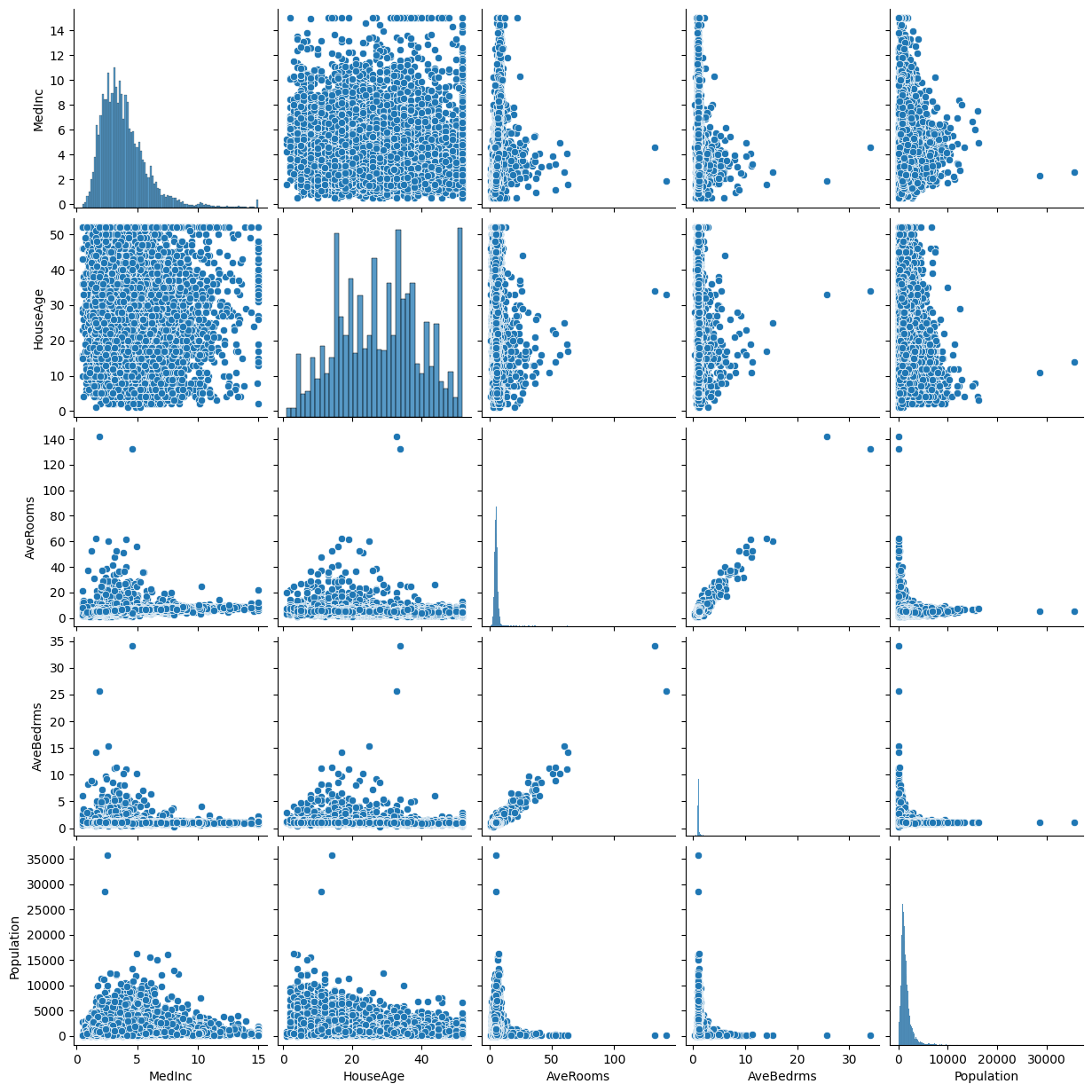
전진 선택법 (Forward Selection)
- 설명변수가 하나도 없는 모델에서 시작하여 가장 유의미한 변수를 하나씩 추가
- 장점
- 간단하고 해석이 용이
- 단점
- 한번 선택된 변수는 제거되지 않음
1
2
3
4
5
6
7
8
9
10
11
12
13
14
15
16
17
18
19
20
21
22
23
24
25
26
27
28
29
30
31
32
33
34
35
36
37
38
 from sklearn.datasets import fetch_california_housing
 from sklearn.linear_model import LinearRegression
 from sklearn.feature_selection import SequentialFeatureSelector, RFE
 import numpy as np
 import pandas as pd
 import seaborn as sns
 import matplotlib.pyplot as plt

 # 데이터 로드
 data = fetch_california_housing()
 X = data.data
 y = data.target

 # 데이터 정보 출력
 print("Feature Names:", data.feature_names)
 print("Data Shape:", X.shape)
 # Feature Names: ['MedInc', 'HouseAge', 'AveRooms', 'AveBedrms', 'Population', 'AveOccup', 'Latitude', 'Longitude']
 # Data Shape: (20640, 8)

 # 모델 초기화
 model = LinearRegression()

 # 전진 선택법
 sfs = SequentialFeatureSelector(model, direction='forward', n_features_to_select=5)
 sfs.fit(X, y)

 # 선택된 Feature
 selected_features = np.array(data.feature_names)[sfs.get_support()]
 print("선택된 Feature:", selected_features)
 # 선택된 Feature: ['MedInc' 'HouseAge' 'AveRooms' 'AveBedrms' 'Population']

 # 데이터프레임 생성
 df = pd.DataFrame(X, columns=data.feature_names)

 # 선택된 Feature 분포 시각화
 selected_df = df[selected_features]
 sns.pairplot(selected_df)
 plt.show()
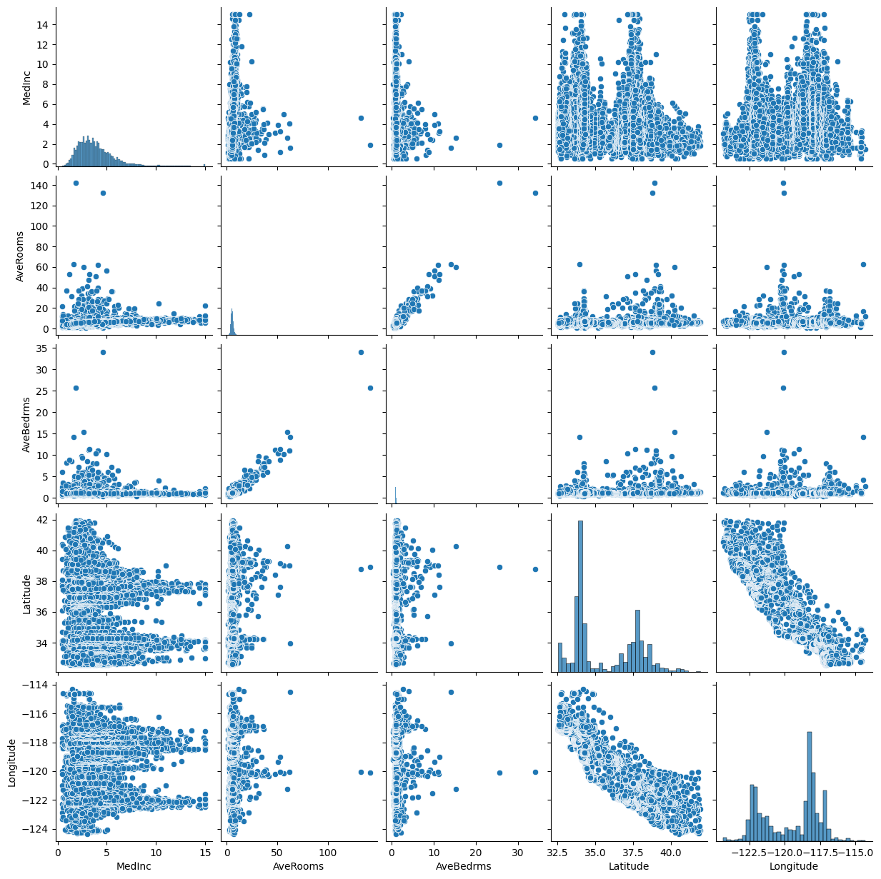
후진 소거법 (Backward Elimination)
- 모든 변수를 사용하여 모델을 시작하고, 유의미하지 않은 변수를 하나씩 제거
- 장점
- 처음에 모든 변수를 고려하여 시작
- 단점
- 한번 제거된 변수는 다시 선택되지 않음
1
2
3
4
5
6
7
8
9
10
11
12
13
14
15
16
17
18
19
 # 모델 초기화
 model = LinearRegression()

 # 후진 소거법
 rfe = RFE(model, n_features_to_select=5)
 rfe.fit(X, y)

 # 선택된 Feature
 selected_features = np.array(data.feature_names)[rfe.support_]
 print("선택된 Feature:", selected_features)
 # 선택된 Feature: ['MedInc' 'AveRooms' 'AveBedrms' 'Latitude' 'Longitude']

 # 데이터프레임 생성
 df = pd.DataFrame(X, columns=data.feature_names)

 # 선택된 Feature 분포 시각화
 selected_df = df[selected_features]
 sns.pairplot(selected_df)
 plt.show()
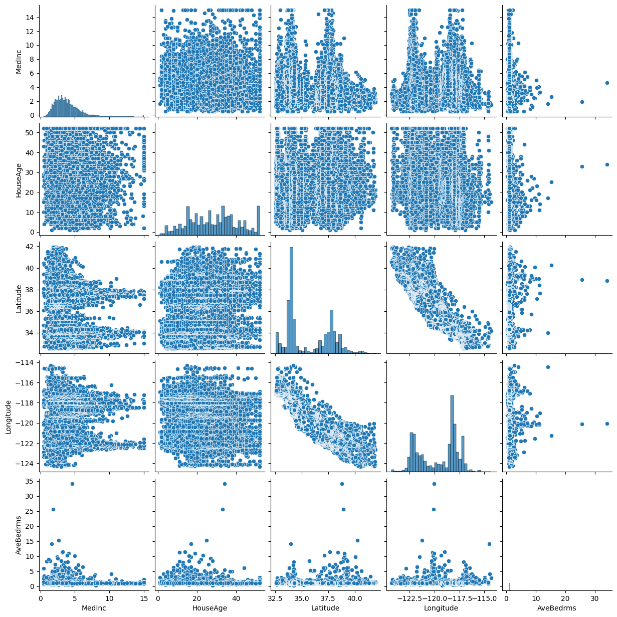
단계적 선택법 (Stepwise Selection)
- 전진 선택법과 후진 소거법을 번갈아 수행하는 기법
- 장점
- 변수 추가와 제거가 모두 가능
- 한번 선택된 변수가 이후 과정에서 제거되거나, 제거된 변수가 이후 과정에서 재선택될 수 있음
- 단점
- 계산 비용이 높을 수 있음
1
2
3
4
5
6
7
8
9
10
11
12
13
14
15
16
17
18
19
20
21
22
23
24
25
26
27
28
29
30
31
32
33
34
35
36
37
38
39
40
 from sklearn.metrics import mean_squared_error

 def stepwise_selection(X, y, model, n_features_to_select):
     remaining_features = list(range(X.shape[1]))
     selected_features = []
     best_score = float('inf')

     while len(selected_features) < n_features_to_select:
         scores = []
         for feature in remaining_features:
             candidate_features = selected_features + [feature]
             model.fit(X[:, candidate_features], y)
             score = mean_squared_error(y, model.predict(X[:, candidate_features]))
             scores.append((score, feature))

         scores.sort()
         best_score, best_feature = scores[0]
         selected_features.append(best_feature)
         remaining_features.remove(best_feature)

     return selected_features

 # 단계적 선택법 실행
 model = LinearRegression()
 selected_features_indices = stepwise_selection(X, y, model, n_features_to_select=5)
 selected_features = np.array(data.feature_names)[selected_features_indices]
 print("단계적 선택법으로 선택된 Feature:", selected_features)
 # 단계적 선택법으로 선택된 Feature: ['MedInc' 'HouseAge' 'Latitude' 'Longitude' 'AveBedrms']

 import pandas as pd
 import seaborn as sns
 import matplotlib.pyplot as plt

 # 데이터프레임 생성
 df = pd.DataFrame(X, columns=data.feature_names)

 # 선택된 Feature 분포 시각화
 selected_df = df[selected_features]
 sns.pairplot(selected_df)
 plt.show()
유전 알고리즘 (Genetic Algorithm, GA)
- 진화론적 개념(자연 선택 및 유전)을 기반으로 최적화를 수행하는 메타 휴리스틱 알고리즘
- 핵심 개념
- 선택 (Selection): 우수한 해를 부모 세대로 선택
- 교배 (Crossover): 부모 세대의 유전자를 교환하여 새로운 세대 생성
- 돌연변이 (Mutation): 낮은 확률로 변이를 발생시켜 Local Optimum에서 탈출
- 적합도 (Fitness): 각 해의 품질을 평가하는 함수
- 절차
- 염색체 초기화 및 하이퍼파라미터 설정
- 각 염색체의 적합도 평가
- 우수 염색체 선택 및 교배 수행
- 돌연변이 적용
- 반복적으로 다음 세대 생성 및 적합도 평가
- 최종 변수 집합 선택
- 장점
- 전역 최적화를 수행하므로, Feature 선택에서 최적의 조합을 찾을 가능성이 높음
- 단점
- 계산 비용이 크며, 하이퍼파라미터(세대 수, 돌연변이율 등)에 민감함
1
2
3
4
5
6
7
8
9
10
11
12
13
14
15
16
17
18
19
20
21
22
23
24
25
26
27
28
29
30
31
32
33
34
35
36
37
38
39
40
41
42
43
44
45
46
47
48
49
50
51
52
53
54
55
56
57
58
59
60
61
62
63
64
65
66
67
68
69
 import random
 import numpy as np
 from sklearn.linear_model import LinearRegression
 from sklearn.model_selection import train_test_split
 from sklearn.metrics import mean_squared_error

 # 데이터 로드
 from sklearn.datasets import fetch_california_housing
 data = fetch_california_housing()
 X = data.data
 y = data.target
 feature_names = data.feature_names

 # 유전 알고리즘 함수
 def genetic_algorithm(X, y, population_size=10, num_generations=50, mutation_rate=0.1):
     num_features = X.shape[1]

     # 초기화: 랜덤 염색체 생성
     population = [np.random.randint(0, 2, num_features) for _ in range(population_size)]

     def fitness(chromosome):
         selected_features = np.where(chromosome == 1)[0]
         if len(selected_features) == 0:
             return float('inf')  # 아무 Feature도 선택되지 않으면 적합도 최악

         X_selected = X[:, selected_features]
         X_train, X_test, y_train, y_test = train_test_split(X_selected, y, test_size=0.2, random_state=42)

         model = LinearRegression()
         model.fit(X_train, y_train)
         predictions = model.predict(X_test)

         return mean_squared_error(y_test, predictions)

     def crossover(parent1, parent2):
         point = random.randint(1, num_features - 1)
         return np.concatenate([parent1[:point], parent2[point:]])

     def mutate(chromosome):
         for i in range(len(chromosome)):
             if random.random() < mutation_rate:
                 chromosome[i] = 1 - chromosome[i]  # 0 <-> 1 변환
         return chromosome

     for generation in range(num_generations):
         # 적합도 평가
         population = sorted(population, key=lambda chromo: fitness(chromo))
         next_generation = population[:population_size // 2]  # 상위 절반 선택

         # 새로운 세대 생성
         while len(next_generation) < population_size:
             parent1, parent2 = random.sample(next_generation, 2)
             child = crossover(parent1, parent2)
             child = mutate(child)
             next_generation.append(child)

         population = next_generation

     # 최적 해 선택
     best_chromosome = min(population, key=lambda chromo: fitness(chromo))
     selected_features = np.where(best_chromosome == 1)[0]
     return best_chromosome, selected_features

 # 실행
 best_chromosome, selected_features = genetic_algorithm(X, y)
 print("Best Chromosome:", best_chromosome)
 print("Selected Features:", np.array(feature_names)[selected_features])
 # Best Chromosome: [1 1 1 0 1 1 1 1]
 # Selected Features: ['MedInc' 'HouseAge' 'AveRooms' 'Population' 'AveOccup' 'Latitude' 'Longitude']
Feature 축소
- 고차원 데이터의 차원을 줄이면서 데이터의 분산(정보)을 최대한 보존
데이터의 주요 패턴을 찾고, 불필요한 차원을 제거하여 모델의 효율성을 높임
주성분 분석 (PCA, Principal Component Analysis)
- 고차원 데이터를 저차원으로 축소하면서 데이터의 분산(정보)을 최대한 보존하는 선형 차원 축소 기법
- 데이터를 새로운 좌표계로 변환하여 데이터의 주요 패턴을 찾고, 불필요한 차원을 제거하는 데 사용
- 예
- 3차원의 데이터를 2차원의 주성분 공간으로 사영(projection) 시키면 원래 데이터가 가지는 특징의 대부분이 보존
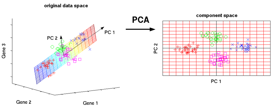
- 원리
- 주성분 (Principal Component)
- 데이터의 분산이 가장 큰 방향을 나타내는 새로운 축을 생성
- PC1: 데이터 분산이 가장 크게 설명되는 축
- PC2: PC1에 직교(90도)하면서 분산이 그 다음으로 큰 방향
- 공분산 행렬 (Covariance Matrix)
- 데이터의 변수들 간의 관계를 표현
- 공분산의 행렬과 고유값, 고유벡터를 사용해 주성분을 정의
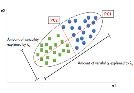
- 고유값 (Eigenvalue, λ)
- 각 주성분이 설명하는 분산의 크기
- 값이 클수록 해당 주성분이 더 중요함을 의미
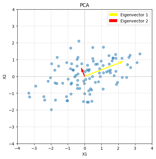
- 고유벡터 (Eigenvector, v)
- 주성분의 방향을 나타내는 단위벡터
- 서로 직교(orthogonal)하는 특성을 가짐
- 데이터를 새로운 좌표계로 변환하는 기저(basis)로 사용
- 고유값 (Eigenvalue, λ)
- 주성분 (Principal Component)
- 과정
- 데이터 정규화: 모든 Feature를 동일한 스케일로 변환
- 공분산 행렬 계산: 데이터 변수 간의 관계를 계산
- 고유값과 고유벡터 계산: 각 주성분의 방향과 중요도 평가
- 주성분 선택: 고유값 크기를 기준으로 중요도가 높은 주성분 선택
- 데이터 사영(Projection): 데이터를 선택된 주성분 축으로 변환
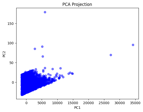
1
2
3
4
5
6
7
8
9
10
11
12
13
14
15
16
17
18
19
20
21
22
23
24
25
26
27
28
from sklearn.datasets import fetch_california_housing
from sklearn.decomposition import PCA
import matplotlib.pyplot as plt
import pandas as pd

# 데이터 로드
california = fetch_california_housing()
X = pd.DataFrame(california.data, columns=california.feature_names)

# PCA 적용
pca = PCA(n_components=2)
transformed_data = pca.fit_transform(X)

# 결과 출력
print("주성분:", pca.components_)
print("설명된 분산 비율:", pca.explained_variance_ratio_)
# 주성분: [[ 8.11734515e-06 -3.29264421e-03 -1.57754708e-04 -2.77006684e-05
#    9.99994324e-01  6.40764448e-04 -2.05179008e-04  1.76522227e-04]
#  [-1.98005360e-02  9.92216370e-01 -3.90115135e-02 -4.23881026e-03
#    3.18858393e-03  1.15585346e-01 -3.52344718e-03 -1.38634158e-02]]
# 설명된 분산 비율: [9.99789327e-01 1.13281110e-04]

# 시각화
plt.scatter(transformed_data[:, 0], transformed_data[:, 1], c='blue', alpha=0.5)
plt.title("PCA Projection")
plt.xlabel("PC1")
plt.ylabel("PC2")
plt.show()
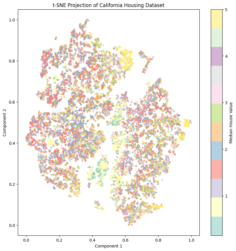
t-SNE (t-Distributed Stochastic Neighbor Embedding)
- 고차원 공간에서 가까운 것은 저차원에서도 가깝게, 고차원에서 먼 것은 저차원에서도 멀게 유지하는 차원 축소 기법
- 비선형 차원 축소 기법으로, 비선형 변환을 사용하여 복잡한 데이터 구조를 효과적으로 표현
데이터 간의 유사성(Similarity)에 중점을 두며, 글로벌 구조(Global Structure)보다 로컬 구조(Local Structure)를 더 잘 반영

- 작동 원리
- 고차원 데이터 유사성 계산
- 데이터 간의 거리 기반 확률 분포 계산
- 저차원 데이터 유사성 계산
- 두 분포 간의 차이 최소화
- Kullback-Leibler Divergence를 최소화
- 데이터 포인트 이동
- 저차원에서 데이터의 위치를 조정하여 구조를 반영
- 고차원 데이터 유사성 계산
- 특징
- 로컬 구조(Local Structure) 보존
- 가까운 데이터 포인트 간의 관계를 최대한 유지하며, 저차원에서도 local 군집 유지
- 글로벌 구조(Global Structure) 표현 약화
- 멀리 떨어진 데이터 포인트 간의 관계는 왜곡될 가능성 있음
- 계산 비용이 높음
- 고차원 데이터가 크면 계산량이 많고 학습 시간이 오래 걸림
- 해석의 어려움
- 결과로 나온 저차원 데이터가 원래 분포를 완벽히 반영하지 않을 수 있음
- 로컬 구조(Local Structure) 보존
1
2
3
4
5
6
7
8
9
10
11
12
13
14
15
16
17
18
19
20
21
22
23
24
25
26
27
28
29
30
31
32
33
34
35
36
37
38
39
40
41
42
43
44
 from sklearn.datasets import fetch_california_housing
 from sklearn.manifold import TSNE
 from sklearn.preprocessing import StandardScaler
 import matplotlib.pyplot as plt
 import pandas as pd
 import numpy as np

 # 데이터 로드
 california = fetch_california_housing()
 X = pd.DataFrame(california.data, columns=california.feature_names)
 y = california.target

 # 데이터 스케일링
 scaler = StandardScaler()
 X_scaled = scaler.fit_transform(X)

 # t-SNE 파라미터 조정
 tsne = TSNE(
     n_components=2,
     perplexity=30,
     random_state=42
 )

 # t-SNE 적용
 transformed_data = tsne.fit_transform(X_scaled)

 # 정규화하여 0-1 범위로 조정
 transformed_normalized = (transformed_data - transformed_data.min(axis=0)) / (transformed_data.max(axis=0) - transformed_data.min(axis=0))

 # 시각화
 plt.figure(figsize=(10, 10))
 scatter = plt.scatter(
     transformed_normalized[:, 0],
     transformed_normalized[:, 1],
     c=y,
     cmap='Set3',
     alpha=0.6,
     s=10  # 점 크기를 작게 조정
 )
 plt.colorbar(scatter, label="Median House Value")
 plt.title("t-SNE Projection of California Housing Dataset")
 plt.xlabel("Component 1")
 plt.ylabel("Component 2")
 plt.show()
Feature 생성 및 변환 후 원래 Feature 삭제 여부
삭제가 적절한 경우
- 변환된 Feature가 정보를 완전히 대체하는 경우
- 고차원 데이터에서 차원을 줄이고 싶은 경우
- 원래 Feature가 노이즈로 작용하는 경우
삭제하지 않는 것이 적절한 경우
- 모델 성능 비교가 필요할 경우
- 원래 Feature의 해석 가능성이 중요한 경우
- 다양한 모델에서 테스트할 계획이 있는 경우
Feature와 모델 성능
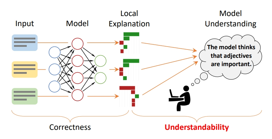
모델 해석의 중요성
모델의 성능만으로 충분하지 않음
- 실제 배포되고 사용되는 시스템은 평가 데이터와 실제 데이터의 분포가 다를 가능성이 있음
- 평가 지표만으로는 모델의 신뢰성을 보장하기 어려움
- 모델 성능을 신뢰하려면 성능 지표 외에도 내부 동작에 대한 이해가 필요
모델 해석은 성능 개선에 도움을 줌
- 모델 내부 작동 원리를 이해함으로써 성능 병목지점 발견 가능
- 특정 Feature의 중요도를 평가하여 불필요한 Feature를 제거하거나 개선점을 도출
모델 결정 이유가 요구되는 상황 존재
- 모델의 해석 가능성은 신뢰도를 높이고, 사용자와의 신뢰를 구축하는 데 필수적
- 예시
- 은행 대출 심사 시스템에서 거절 사유를 설명할 필요가 있음
Feature 선택 및 중요도 평가
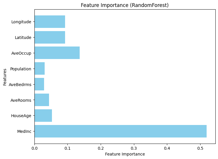
Feature Importance (특성 중요도)
- 각 Feature가 예측에 얼마나 기여했는지 평가
- 주로 트리 기반 모델(Random Forest, XGBoost 등)에 사용
- 불순도 감소 기준(Gini Impurity, Entropy 등)을 활용해 중요도를 계산
- Feature의 중요도를 상대적인 값으로 제공
- 장점
- 빠른 계산
- 모델 학습 과정에서 자동으로 중요도를 계산
- 직관적 해석
- 중요도가 높은 Feature를 바로 식별 가능
- 빠른 계산
- 단점
- Feature 간 상관성 문제
- 높은 상관관계가 있는 Feature가 왜곡된 중요도를 가질 수 있음
- 특정 모델에 의존
- 선형 모델에서는 직접적인 계산이 어려움
- Feature 간 상관성 문제
1
2
3
4
5
6
7
8
9
10
11
12
13
14
15
16
17
18
from sklearn.ensemble import RandomForestRegressor
import matplotlib.pyplot as plt
import pandas as pd

# 랜덤 포레스트 모델 학습
model = RandomForestRegressor(random_state=42)
model.fit(X, y)

# Feature Importance 계산
importance = model.feature_importances_

# 시각화
plt.figure(figsize=(8, 6))
plt.barh(X.columns, importance, color="skyblue")
plt.xlabel("Feature Importance")
plt.ylabel("Features")
plt.title("Feature Importance (RandomForest)")
plt.show()
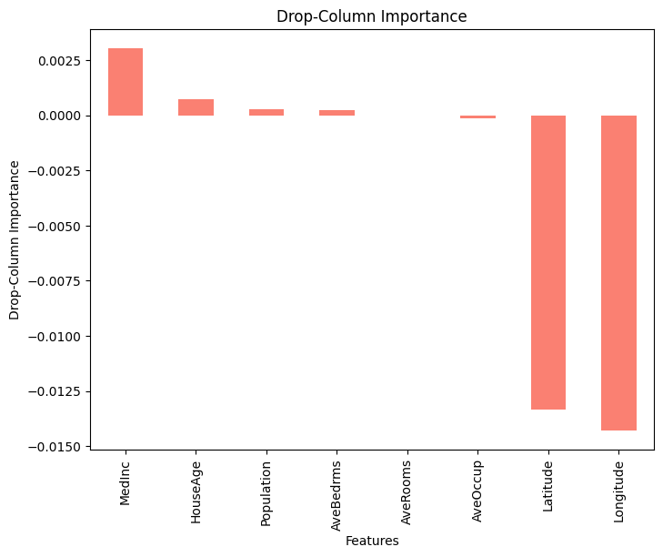
Drop-Column Importance
- Feature를 하나씩 제거하고 모델 성능 변화를 측정하여 중요도를 평가
- 각 Feature의 중요도를 직접적으로 확인 가능
- 장점
- 모델 독립성
- 모델 종류에 상관없이 적용 가능
- 정교한 중요도 계산
- 실제 성능 차이를 기반으로 중요도를 측정하므로 신뢰도가 높음
- 모델 독립성
- 단점
- 계산 비용이 높음
- 각 Feature마다 모델 재학습이 필요
- 데이터 의존성
- 작은 데이터셋에서 Feature를 제거하면 과소 평가될 가능성 존재
- 계산 비용이 높음
- 예시
- “type” Feature를 제거했을 때 성능 차이가 크다면 해당 Feature는 모델 성능에 가장 중요한 변수
1
2
3
4
5
6
7
8
9
10
11
12
13
14
15
16
17
18
19
20
21
from sklearn.metrics import mean_squared_error

# Drop-Column Importance 계산
baseline_mse = mean_squared_error(y, model.predict(X))

drop_importances = {}
for feature in X.columns:
   X_dropped = X.drop(columns=[feature])
   model.fit(X_dropped, y)
   mse = mean_squared_error(y, model.predict(X_dropped))
   drop_importances[feature] = baseline_mse - mse

# 결과 정렬 및 시각화
drop_importances = pd.Series(drop_importances).sort_values(ascending=False)

plt.figure(figsize=(8, 6))
drop_importances.plot(kind="bar", color="salmon")
plt.xlabel("Features")
plt.ylabel("Drop-Column Importance")
plt.title("Drop-Column Importance")
plt.show()
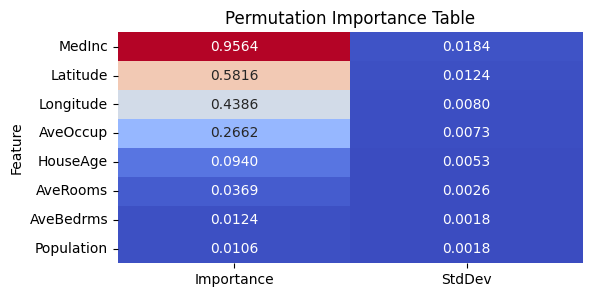
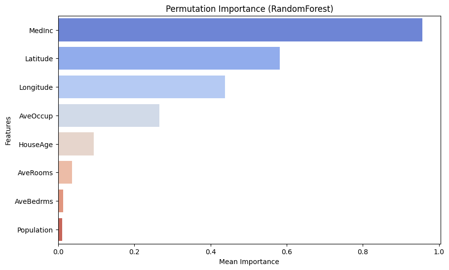
Permutation Importance
- 모델 학습 후 Feature 값을 랜덤으로 섞어 모델 성능 변화를 측정
- 성능 변화가 클수록 해당 Feature의 중요도가 높다고 평가
- 장점
- 모델 독립성
- 어떤 모델에서도 적용 가능
- 상관성 문제 완화
- 상관성이 없는 Feature에 대해 독립적으로 중요도 평가 가능
- 모델 독립성
- 단점
- 계산 비용
- 반복 평가로 인해 시간이 오래 걸릴 수 있음
- 랜덤성
- 섞기 방식에 따라 결과가 다소 변동될 수 있음
- 계산 비용
1
2
3
4
5
6
7
8
9
10
11
12
13
14
15
16
17
18
19
20
21
22
23
24
25
26
27
28
29
30
31
32
33
34
35
36
37
38
39
40
41
42
43
44
45
46
47
48
49
50
51
52
53
54
55
56
57
58
59
60
61
62
63
64
import numpy as np
import pandas as pd
from sklearn.ensemble import RandomForestRegressor
from sklearn.inspection import permutation_importance
from sklearn.datasets import fetch_california_housing
from sklearn.model_selection import train_test_split
from sklearn.preprocessing import StandardScaler
import matplotlib.pyplot as plt
import seaborn as sns

# 데이터 로드 및 전처리
california = fetch_california_housing()
X = pd.DataFrame(california.data, columns=california.feature_names)
y = california.target

# 데이터 분할 및 스케일링
X_train, X_test, y_train, y_test = train_test_split(X, y, test_size=0.2, random_state=42)
scaler = StandardScaler()
X_train_scaled = scaler.fit_transform(X_train)
X_test_scaled = scaler.transform(X_test)

# RandomForest 모델 학습
model = RandomForestRegressor(random_state=42)
model.fit(X_train_scaled, y_train)

# Permutation Importance 계산
perm_importances = permutation_importance(
   model,
   X_test_scaled,
   y_test,
   scoring='neg_mean_squared_error',
   n_repeats=10,
   random_state=42,
)

# 결과를 DataFrame으로 변환
perm_df = pd.DataFrame({
   "Feature": X.columns,
   "Importance": perm_importances.importances_mean,
   "StdDev": perm_importances.importances_std
}).sort_values(by="Importance", ascending=False)

# 중요도 테이블 출력
print(perm_df)

# 테이블 시각화
plt.figure(figsize=(10, 6))
sns.barplot(data=perm_df, x="Importance", y="Feature", palette="coolwarm", ci=None)
plt.title("Permutation Importance (RandomForest)")
plt.xlabel("Mean Importance")
plt.ylabel("Features")
plt.show()

# 테이블 스타일로 저장
plt.figure(figsize=(6, 3))
sns.heatmap(
   perm_df.set_index("Feature").style.format("{:.4f}").background_gradient(cmap="coolwarm").data,
   annot=True,
   fmt=".4f",
   cmap="coolwarm",
   cbar=False
)
plt.title("Permutation Importance Table")
plt.show()
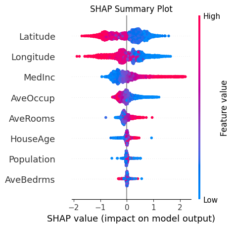
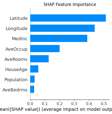
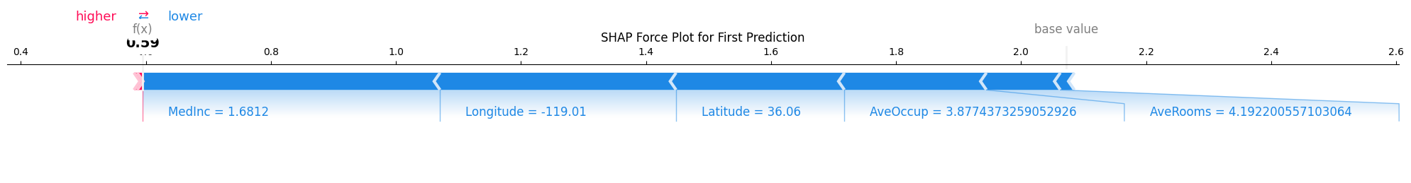
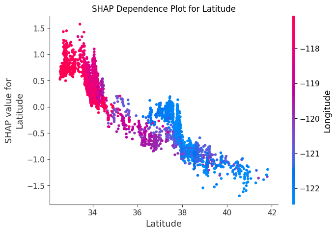
SHAP (Shapley Additive exPlanations)
- 게임 이론의 Shapley 값 기반으로 각 Feature가 모델 예측에 미친 영향을 공정하게 평가
- Feature를 포함했을 때와 포함하지 않았을 때의 모델 출력 변화를 계산하여 기여도를 평가
- 장점
- 어떤 모델에도 적용 가능
- Feature 간 상호작용을 고려하여 정확한 기여도 계산
- 글로벌 해석
- 모델 전체에서 중요한 Feature 확인
- 로컬 해석
- 특정 예측값에 대해 각 Feature의 기여도를 분석
- 단점
- 조합을 반복적으로 평가해야 하므로 비용이 높음
- 스케일링 여부에 따라 결과가 달라질 수 있음
- 상호작용 분석이 복잡할 수 있음
- 수식 : \(f(x) = \phi_0 + \sum_{i=1}^M \phi_i\)
- \(f(x)\): 모델의 예측값
- \(\phi_0\): 기본값 (base value)
- \(\phi_i\): Feature i의 Shapley 값
- \(M\): Feature의 총 개수
1
2
3
4
5
6
7
8
9
10
11
12
13
14
15
16
17
18
19
20
21
22
23
24
25
26
27
28
29
30
31
32
33
34
35
36
37
38
39
40
41
42
43
44
45
46
47
48
49
50
51
52
53
54
55
56
57
58
import shap
import xgboost as xgb
from sklearn.datasets import fetch_california_housing
from sklearn.model_selection import train_test_split
import matplotlib.pyplot as plt
import numpy as np

# 데이터 준비
california = fetch_california_housing()
X = california.data
y = california.target
feature_names = california.feature_names

# 데이터 분할
X_train, X_test, y_train, y_test = train_test_split(X, y, test_size=0.2, random_state=42)

# XGBoost 모델 학습
model = xgb.XGBRegressor(random_state=42)
model.fit(X_train, y_train)

# SHAP 값 계산
explainer = shap.TreeExplainer(model)
shap_values = explainer.shap_values(X_test)

# 다양한 SHAP 시각화
plt.figure(figsize=(20, 10))

# Summary Plot
plt.subplot(121)
shap.summary_plot(shap_values, X_test, feature_names=feature_names, show=False)
plt.title("SHAP Summary Plot")
plt.tight_layout()
plt.show()

# Bar Plot
plt.subplot(122)
shap.summary_plot(shap_values, X_test, feature_names=feature_names, plot_type="bar", show=False)
plt.title("SHAP Feature Importance")

plt.tight_layout()
plt.show()

# Force Plot (첫 번째 예측에 대한 로컬 설명)
plt.figure(figsize=(12, 4))
shap.force_plot(explainer.expected_value, shap_values[0,:], X_test[0,:],
              feature_names=feature_names, matplotlib=True, show=False)
plt.title("SHAP Force Plot for First Prediction")
plt.tight_layout()
plt.show()

# Dependence Plot (가장 중요한 특성에 대해)
shap_abs_mean = np.abs(shap_values).mean(axis=0)
most_important_feature_idx = shap_abs_mean.argmax()
plt.figure(figsize=(10, 6))
shap.dependence_plot(most_important_feature_idx, shap_values, X_test,
                  feature_names=feature_names, show=False)
plt.title(f"SHAP Dependence Plot for {feature_names[most_important_feature_idx]}")
plt.show()
Reference
- https://www.heavy.ai/technical-glossary/feature-engineering
- https://www.youtube.com/watch?v=bEX6WPMiLvo
- https://mltechniques.com/2022/05/17/new-book-approaching-almost-any-machine-learning-problem/
- https://www.aitimes.kr/news/articleView.html?idxno=24963
- https://towardsdatascience.com/using-shap-values-to-explain-how-your-machine-learning-model-works-732b3f40e137
This post is licensed under CC BY 4.0 by the author.